Tutorial 1: Creating and Solving Factor Graphs

In this tutorial you will learn how to create, solve, and explore factor graphs, as well as what variables, factors, and priors are.

API Version: NavAbilitySDK.py

YouTube Walk Through Video:

You can follow along with a YouTube walk through recording of this Tutorial notebook:

Application of this Tutorial

These tutorials apply broadly to “robotics”, and it is worth noting that we define ‘robotics’ to include

• Infrastructure Management: Digitize construction, manufacturing, warehousing operations into real-time virtual assets

• Warehouse Automation: Orchestrating interactions between pickers and AGVs in a warehouse

• Enhanced metrology and calibration equipment.

• Environment mapping and survey equipment, including cell phone survey, robotic surveyor Total Station.

• Inspection and monitoring robots building a map (factory, warehouses, subsea infrastructure, etc.)

• And many more.

Vision: Interacting Robotics

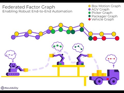
Zooming in further, let’s consider a factory environment where various interacting robotic equipment are producing and transporting objects – i.e. manufacturing and logistics support. The figure below conceptually shows how a product winds it’s way from the factory floor, through various robotic handovers, and out via shipping on a truck. Each robot individually needs a geometrical (and later semantic) understanding of the task object, their location, the surroundings, and of other agents. Each robot therefore will have it’s own navigation solution.

Longer term, these navigation solutions will need to interact. The figure below shows at the highest level how factor graphs provide a technique / method / roadmap on how to develop more intelligent robotic equipment that can calibrate, localize, map, track, interact, or cooperate:

This tutorial starts the conversation on how to overcome the crux navigation AI software challenge, and applies to both individual and interacting robotic systems. This tutorial is the first step in showing how the idea of factor graphs can provide a good engineering balance in flexibility, ease of use, and mathematical foundation.

This tutorial will show some of the most basic operations that you can perform with factor graphs, and further tutorials will fill in more and more of the features and capabilities. Keep in mind that this and several more tutorials must be brought together for the necessary feature set to deploy multi-agent environments of interacting humans and robots.

ICRA Survey

Thanks for doing our tutorials! We really want to make sure this is valuable for you.

This quick 2 minute survey will help us improve them for next year’s workshop.

What is a Factor Graph

Calibration / localization / tracking / mapping / perception problems in robotics can be solved very effectively with factor graphs, which provide a common language to describe the underlying estimation problem from available data; and in a way both humans and computers can easily understand. A factor graph is a graphical modelling language with two types of nodes, namely variables and factors, which are connected by edges according to how they interact. This sketch illustrates a simple example with variables, the large circular nodes, and factors, the square nodes – note, the interactive code segments below will explain how graphs this like are constructed and why:

Variables represent unknown states that the user wants the computer to estimate, such as the position or orientation of some equipment, or position of landmarks in the environment, or maybe hidden calibration parameters that are difficult to measure directly, and potetially many, many more.

Factors usually represent the interaction between sparse variables based on some measurement data, e.g. the distance from one point to another – i.e. a range factor. This is where basic math and measurement functions are included and used during computation. For example, encoder measurements from wheels, ranges from a laser, or tag readings from a camera. The variables associated with each data cue / measurement is depicted by the edges eminating from each factor. Our solution aleady provides a library of standard variables and factors that require zero mathematical input from the user, yet the technology rapidly supports building of new variables and factors, potentially containing exotic computations – more on that later.

From a technical perspective, factor graphs allow for an apples and apples framework where different sensor measurements / data cues can be combined and jointly processed according to their indivual statistical properties. Factor graphs allow the system developer to think about each measurement on their own, rather than having to deal with the challenging data fusion problem manually. This greatly simplifies the problem, since the rigorous computational aspects are dealt with by factor graph solver and associated algorithms.

Later tutorials will show how to handle low confidence, ambiguous, and ‘strange’ measurement scenarios. This is an interactive tutorial, so let’s dive in and navigate a robot!

For additional info, see the Caesar.jl docs on Graph Concepts and beyond, for more details on graph factorization, elimination, recycling, federated solutions, data handling, serialization and much more.

Loading the Packages

First we will need some packages:

• NavAbilitySDK - for interacting with the graph.

• numpy - for matrices and calculations.

# # ONLY IF REQUIRED, Install a pip package in the current Jupyter kernel
# import sys
# !{sys.executable} -m pip install navabilitysdk

from navability.entities import *
from navability.services import *
from uuid import uuid4
import asyncio
import numpy as np

Build a factor graph

To create a new factor graph with default settings create a new NavAbility client and a client that indicates the user, robot, and session.

# Start with an empty factor graph
navability_client = NavAbilityHttpsClient()
client = Client("guest@navability.io", "SDKpy_" + str(uuid4())[0:4], "Tutorial1_" + str(uuid4())[0:4])
print(client)

Variables and Factors

Variables represent state variables of interest such as vehicle or landmark positions, sensor calibration parameters, and more. Variables are likely hidden values that are not directly observed, but we want to estimate them from observed data and at least some minimal algebra structure from probabilistic measurement models.

Factors represent the interaction between particular variables, as captured measurement or data cues. For example, a distance travelled measurement between two pose variables. Relative factors between variables are probabilistic models that capture the likelihood interactions between variables. Priors factors (i.e. unary to one variable) represent absolute information to be introduced about that variable, for example a GPS measurement; more on how to introduce distrust of such priors later.

NavAbilitySDK.py provides variables and factors useful to robotics. We start with a Pose2 variable, i.e. position and orientation in two dimensions. To add variables to our factor graph we created above, call addVariable with a label x0 and type Pose2

result_id = await addVariable(navability_client, client, "x0", VariableType.Pose2)
print(f"Added x0 with result ID {result_id}")
# Wait for it to be loaded.
await waitForCompletion(navability_client, [result_id])

We now have a factor graph with one variable, but to solve it we need some additional information. In this example, we need the estimated starting point of our robot. We use unary factors called priors to represent absolute information to be introduced. In this case we use PriorPose2, as our variable type is also Pose2. This unary factor is taken as a matrix FullNormal distribution (a.k.a. a multivariate normal distribution). Let’s create a PriorPose2 unary factor with zero mean and a covariance matrix of (diagm([0.05,0.05,0.01].^2)):

\(\mu = \begin{bmatrix} 0 & 0 & 0 \end{bmatrix}^T\)

\(\Sigma = \begin{bmatrix} 0.0025 & 0.0 & 0.0 \\ 0.0 & 0.0025 & 0.0 \\ 0.0 & 0.0 & 0.0001 \end{bmatrix}\)

prior_distribution = FullNormal(mu=np.zeros(3), cov=np.power(np.diag([0.1, 0.1, 0.1]),2))
result_id = await addFactor(navability_client, client, ["x0"], PriorPose2(Z=prior_distribution)) 
print(f"Added factor with result ID {result_id}")
# Wait for it to be loaded.
await waitForCompletion(navability_client, [result_id])

We can look at the factor graph we have so far using the generated link to the NavAbilityApp, and note the variable node x0 and prior factor node x0f1.

# click the generated graphic to link to the NavAbiltiy WebApp visualization
GraphVizApp(client, variableStartsWith="")

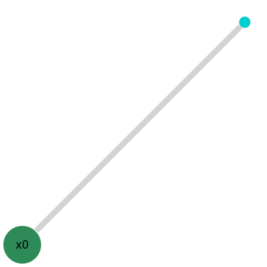
The prior is now connected to the variable, x0, but it is not initialized yet. Automatic initialization of variables depends on how the factor graph model is constructed. So far, x0 has not been initialized.

Graph-based Initialization

At this stage x0 is not initialized, since no numerical solution has yet been computed. We do this as the future intentions of the user are unknown and the initialization of x0 is deferred until the latest possible moment. The NavAbility Platform assumes that the new variables and factors can be initialized when they are solved for the first time.

By delaying initialization of a new variable (say x0) until a second newer uninitialized variable (say x1) that depends on x0, the Caesar.jl algorithms can initialize x0 with more information from surrounding variables and factors. Solving over the entire graph will set the numerical values.

Robot Odometry - Relative Factor

Next, we want to add an odometry factor that connects our two robot poses x0 and x1 together to form a chain. Here we use a relative factor of type Pose2Pose2 with a measurement from pose x0 to x1 of (x=1.0,y=0.0,θ=pi/2); the robot drove 1 unit forward (in the x direction). Similarly to the prior we added above, we use a FullNormal distribution to represent the odometry with mean and covariance:

\(\mu =(x=1, y=0, \theta=\frac{\pi}{2})\)

\(\Sigma = \begin{bmatrix} 0.01 & 0.0 & 0.0 \\ 0.0 & 0.01 & 0.0 \\ 0.0 & 0.0 & 0.0001 \end{bmatrix}\)

result_v = await addVariable(navability_client, client, "x1", VariableType.Pose2)
print(f"Added x1 with result ID {result_v}")
odo_distribution = FullNormal(mu=[1.0, 0.0, np.pi/2], cov=np.power(np.diag([0.1, 0.1, 0.01]),2))
result_fac_1 = await addFactor(navability_client, client, ["x0", "x1"], Pose2Pose2(Z=odo_distribution)) 
print(f"Added factor with result ID {result_fac_1}")

# Wait for it to be loaded.
await waitForCompletion(navability_client, [result_v, result_fac_1])

Solving

We now have a graph we can solve using the Multi-Modal iSAM (MM-iSAM) algorithm. The default solver will perform non-parametric inference/state-estimation over our newly created graph.

Fundamentally, inference is performed via the Bayes (junction) tree where Chapman-Kolmogorov transit integral solutions are based on marginal-joint belief estimation (a sum-product / belief-propagation approximation algorithm). Many benefits such as clique recycling are also available. See the Solving Graphs section in the documentation for more detail.

solve_request = await solveSession(navability_client, client)
print('running solve...')

While the solve is processing, let’s look at the factor graph structure again:

# click the generated graphic to link to the NavAbiltiy WebApp visualization
GraphVizApp(client)

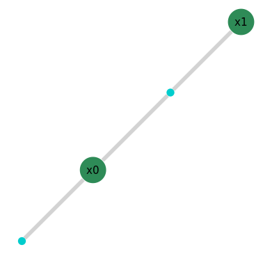
A slightly more the mathy explination. A factor graph represents the factorization of the overall joint probability belief function that describes your system. It represents a breakdown of the complex problem describing your robot navigation, and does so in a way that a computer can work through in a very efficient manner. This factorization allows us to solve the optimization (a.k.a. inference) problem for all variables given every measurement described by the factors.

Multi-Sensor Data Fusion

In our example so far, the graph models the position and orientation (pose) of your robot at any given time, and soon we will add relative measurements to landmarks using a different sensor but captured in the same factor graph.

Results

The NavAbility WebApp allows visualization of the belief state over any of the variables. Also try with Belief and Distribution buttons to see more of the underlying posterior marginal belief estimates.

# Wait for it to be loaded, the very first solve might be slower as some JIT compiling may occur
await waitForCompletion(navability_client, [solve_request], maxSeconds=120)

# click the generated graphic to link to the NavAbiltiy WebApp visualization
MapVizApp(client)

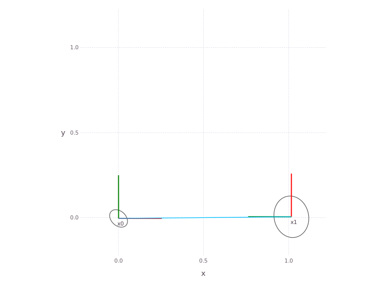
In the App visualization, use the SHOW BELIEF button to see the underlying variable estimates in more detail.

What is happening

The figure shows the position and orientation (red forward) for poses x0 and x1. As well as the covariance ellipse. Since the solver used was non-parametric, the covariance ellipse is based on a best Gaussian distribution fit of the full belief. A few other functions are also handy for interacting with the factor graph, for instance getVariable returns the full variable. Or if you are interested in the suggested Parametric Point Estimate (PPE) you can get this from the PPE data.

variables = await ls(navability_client, client)
print(f"Variables in graph: {variables}")
ppes = {
        v: (await getVariable(navability_client, client, v)).ppes["default"].suggested
        for v in variables
    }
print(ppes)

Parametric point estimates and beliefs

A PPE can be the maximum or mean of the belief. If the belief is a normal distribution, both correspond with its mean. However, care should be taken with using PPEs when beliefs might be non-parametric, for example, in a multimodal belief with two peaks, max corresponds with the maximum of the two peaks while the mean will fall somewhere in between them. In non-parametric cases, it is better to work with the full belief obtained by the Kernel Density Estimate (KDE).
Kernel Density Estimation is a non-parametric way to estimate the probability density function of a random variable. With the default solver, a full probability density function is always available and can be visualized as shown by the distribution plot feature in the NavAbility WebApp. Non-parametric solutions will be discussed in more detail in tutorial 2.

More plotting options exist, depending on how you are accessing the data. See the section on Plotting in the Caesar docs for additional detail.

Adding A Landmark from a Different Sensor

So far we worked with the Pose2 factor type. Among others, NavAbilitySDK also provides the Point2 variable and Pose2Point2BearingRange factor types, which we will use to represent a landmark sighting in our factor graph. We will add a landmark l1 with bearing range measurement of bearing=\((\mu=0,\sigma=0.03)\) range=\((\mu=0.5,\sigma=0.1)\) and continue our robot trajectory by driving around in a square.

results_variables = [
  await addVariable(navability_client, client, "l1", VariableType.Point2),
  await addVariable(navability_client, client, "x2", VariableType.Pose2),
  await addVariable(navability_client, client, "x3", VariableType.Pose2),
  await addVariable(navability_client, client, "x4", VariableType.Pose2)]
results_variables

results_factors = [
  await addFactor(navability_client, client, ["x0", "l1"], Pose2Point2BearingRange(Normal(0.0,0.03), Normal(0.5,0.1))),
  await addFactor(navability_client, client, ["x1", "x2"], Pose2Pose2(odo_distribution)),
  await addFactor(navability_client, client, ["x2", "x3"], Pose2Pose2(odo_distribution)),
  await addFactor(navability_client, client, ["x3", "x4"], Pose2Pose2(odo_distribution)),
]
await waitForCompletion(navability_client, results_variables + results_factors)

Lets go look at the factor graph now, again using the NavAbilityApp

# click the generated graphic to link to the NavAbiltiy WebApp visualization
GraphVizApp(client)

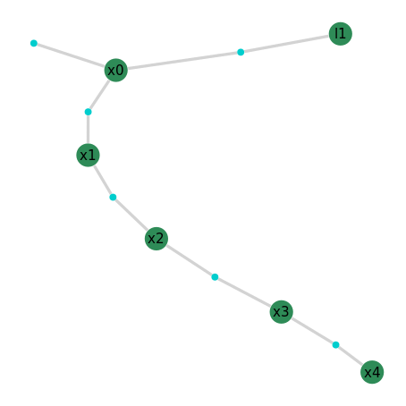
We now have a longer odometry chain with one landmark sighting, let’s solve the factor graph again so we can have a look at the results.

solve_request = await solveSession(navability_client, client)
print('running solve...')
# Wait for it to be loaded.
await waitForCompletion(navability_client, [solve_request], maxSeconds=120)

The solve will take a bit of time. Just keep watching the geometric visualization, which will automatically update as more of the solution is published

# click the generated graphic to link to the NavAbiltiy WebApp visualization
MapVizApp(client)

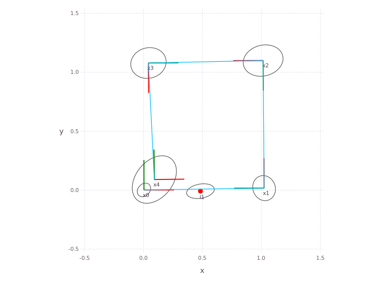
Once solving has completed, the variable results can be looked at in various ways. Here we are just looking at the PPE values, but the full posterior marginal beliefs are available by simply asking for more results.

#pl = plotSLAM2D(fg, drawContour=false, drawEllipse=true, drawhist=false, drawPoints=false)
# TODO: Need l1 to solve for this to work correctly.
variables = await ls(navability_client, client)
print(f"Variables in graph: {variables}")
ppes = {
        v: (await getVariable(navability_client, client, v)).ppes.get("default").suggested
        for v in variables
    }
print(ppes)

Adding a Loop Closure

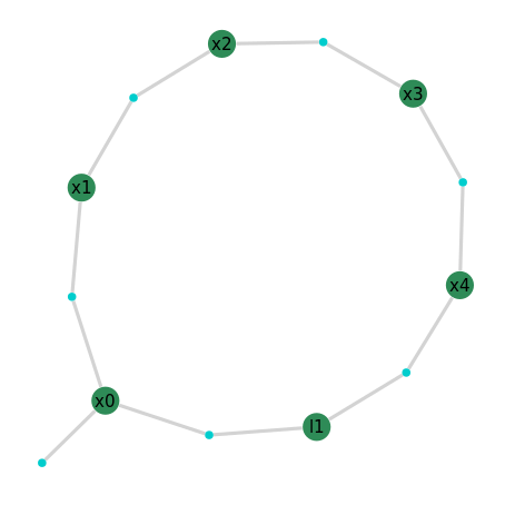
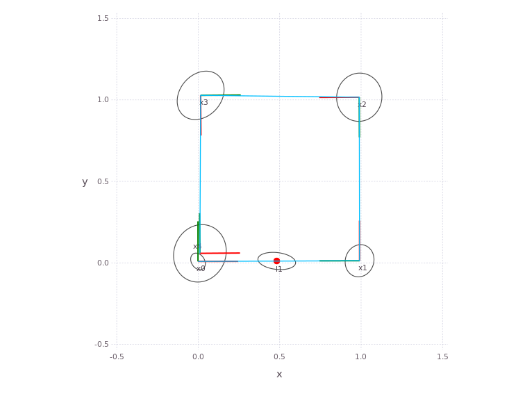
As expected, the robot continued its square trajectory to end off where it started. To illustrate a loop closure, we add another bearing range sighting to from pose x4 to landmark l1, solve the graph and plot the new results:

result_factor = await addFactor(navability_client, client, ["x4", "l1"], Pose2Point2BearingRange(Normal(0.0,0.03), Normal(0.5,0.1)))
await waitForCompletion(navability_client, [result_factor])

solve_request = await solveSession(navability_client, client)
print('running solve...')

Lets go look at the final results again, which now includes the loop closure. Use the ‘Show Belief’, ‘Show Distribution’ buttons along the bottom for more visual information. You can also trigger new solves (as long as the Global Filter fields are properly set in the far right filter menu).

Use the NavAbilityApp hamburger menu on the left to navigate between the graph and geometric map visualization. You can also use the Global Filter menu on the right to set which information to visualize.

# click the generated graphic to link to the NavAbiltiy WebApp visualization
GraphVizApp(client)

# Wait for it to be loaded.
await waitForCompletion(navability_client, [solve_request], maxSeconds=180)

# click the generated graphic to link to the NavAbiltiy WebApp visualization
MapVizApp(client)

Batch parametric solver

NavAbility also provides a parametric batch solver for factor graphs containing only Normal distributions as in this Tutorial. See the Caesar-api/icra-1-simple.ipynb notebook section “Using the parametric solver” for an example of how to use it.

Next Steps

Tutorial 2 will give an introduction to non-parametric solutions.

Additional Resources

Factors are On-Manifold

The variables used in this tutorial, Point2 and Pose2, are represented as points on manifolds and all algebraic operations, inference/optimization are also performed on manifold. For more information on how manifolds are used in Caesar.jl, refer to the manifold section in the documentation.

Custom Variables and Factors

In most scenarios, the existing variables and factors should be sufficient for most robotics applications. Caesar however, is extensible and allows you to easily incorporate your own variable and factor types for specialized applications.

Have a look at the Caesar documentation if you are interested in creating custom variables, factors (or priors)

• Custom variables

• Custom prior factors

• Custom relative factors

Bayes (Junction) Tree

Inference is performed on the Bayes tree see: Bayes tree principles