Tutorial 5: Less Time Wrangling Data, More Time Understanding/Actioning it#
API Version: JuliaLang NavAbilitySDK.py
YouTube Walk Through Video#
A walk through of this video has been prepared and can be found at:
Introduction#
NavAbility developed a case study for marine vehicle navigation which direclty addresses GPS-denied navigation from radar point cloud data. The underlying SLAM solver is supported by NavAbility as open core software. Links to the open source code and deeper discussions are available by following links from Marine Case Study Blog post.
This tutorial shows how interaction is done with ease and efficiency. This tutorial builds on previous tutorials that show how and why factor graphs are so important, as well other tutorials showing some of the robust (non-Gaussian) solver features that are available when building multi-sensor navigation and mapping systems that must combine challenging, ambiguous, and contradictory measurements and data cues.
Problem Statement#
Marine operations in harbor and populated river environments will see increased autonomy with major benefits for safety and efficacy, but the navigational environment poses a number of vital challenges. In developing and testing proof-of-concept systems, four very specific challenges arose:
GPS data can occasionaly drop out, specifically when maneuvering under bridges or between tall structures;
Various perception sensors each perform really well with reasonable availability for seeing obstacles or aiding navigation, but no one sensor alone provides a home run solution;
Practical development testing an operations produces large amounts of recorded robot data, but the data quickly becomes overwhelming and difficult to action;
How to share / integrate measurement data and navigation between agents (human or autonomous), as well as with shore side operations;
The Value (Broader Application)#
By being able to rapidly develop advanced multi-sensor perception, localization, and mapping ideas drastically reduces the cost and risk of introducing highly focussed autonomy/safety features into existing operations.
Access to both raw data and actionable SLAM results provides a major platform for machine learning tasks, such as training predictors that have either geometric of semantic relevance – e.g. learning vehicle behaviors or better classifiers.
Access to a temporal/spatial database allows various sessions to be brought together with NavAbility’s map merging technology.
A Marine SLAM Solution#
The marine case study shows benefits value of persistent simultaneous localization and mapping SLAM solutions.
Raw Data -------------> SLAM Solving ----------------> Action / Visualize Results
              ^                              |
              |                              |
        Enhance the  <--------------- Deeper processing of data
        factor graph                    with previous results
The Data is Alive and Available#
Shows a piece of the boat trajectory. The interactive code below will help visualize the trajectory of the target boat, which was estimated from our vehicle regardless of whether GPS was working or not!
The first piece of code shows:
the factor graph exists
the size of the factor graph
which variables and factors are in the factor graph
In the sections hereafter, you will learn more about which data is being stored in each of these graph nodes, how the SLAM solution is processed and why that is crucial for multisensor navigation, and how to immediately interact the data on the platform for youself.
ICRA Survey#
Thanks for doing our tutorials! We really want to make sure this is valuable for you.
This quick 2 minute survey will help us improve them for next year’s workshop.
Loading Necessary Packages#
Load the necessary packages or accesing the data:
# # ONLY IF REQUIRED, Install a pip package in the current Jupyter kernel
# import sys
# !{sys.executable} -m pip install navabilitysdk
from navability.entities import *
from navability.services import *
from uuid import uuid4
import asyncio
import numpy as np
from PIL import Image as PILImage
from IPython.display import Image
import json
Large Data Blobs#
The solution supports storing large data blobs, which might be associated with zero or more variables in a factor graph.
List Data Entries#
Data blobs can be associated with a variable:
x9_de = await listBlobEntries(client, context, "x9")
for x in x9_de:
  print(x.label)
IMG_CENTER_x11_21827
IMG_CENTER_x11_21829
IMG_CENTER_x11_21837
IMG_CENTER_x13_21867
IMG_CENTER_x9_21806
IMG_CENTER_x12_21851
IMG_CENTER_x12_21848
IMG_CENTER_x13_21862
IMG_CENTER_x11_21840
IMG_CENTER_x12_21852
IMG_CENTER_x13_21863
IMG_CENTER_x11_21826
IMG_CENTER_x12_21842
IMG_CENTER_x10_21813
IMG_CENTER_x10_21817
IMG_CENTER_x9_21797
IMG_CENTER_x10_21818
IMG_CENTER_x10_21819
IMG_CENTER_x11_21838
IMG_CENTER_x10_21816
IMG_CENTER_x10_21822
IMG_CENTER_x11_21831
IMG_CENTER_x11_21833
radar_mkd_full
IMG_CENTER_x9_21809
IMG_CENTER_x13_21861
IMG_CENTER_x9_21799
IMG_CENTER_x10_21821
radar_img
IMG_CENTER_x11_21839
radar_pointcloud
IMG_CENTER_x12_21841
IMG_CENTER_x13_21860
IMG_CENTER_x12_21849
IMG_CENTER_x9_21803
IMG_CENTER_x9_21802
IMG_CENTER_x12_21854
IMG_CENTER_x12_21853
IMG_CENTER_x10_21815
IMG_CENTER_x10_21823
IMG_CENTER_x12_21850
IMG_CENTER_x13_21865
IMG_CENTER_x9_21805
IMG_CENTER_x10_21811
IMG_CENTER_x12_21847
IMG_CENTER_x13_21858
IMG_CENTER_x13_21866
IMG_CENTER_x11_21830
IMG_CENTER_x9_21800
IMG_CENTER_x9_21796
IMG_CENTER_x11_21834
IMG_CENTER_x12_21855
IMG_CENTER_x12_21843
IMG_CENTER_x10_21812
IMG_CENTER_x11_21835
IMG_CENTER_x9_21801
IMG_CENTER_x9_21804
IMG_CENTER_x13_21857
IMG_CENTER_x11_21832
IMG_CENTER_x9_21798
IMG_CENTER_x12_21845
IMG_CENTER_x13_21859
IMG_CENTER_x11_21836
IMG_CENTER_x12_21856
IMG_CENTER_x12_21846
IMG_CENTER_x9_21810
IMG_CENTER_x10_21814
IMG_CENTER_x10_21820
IMG_CENTER_x13_21864
IMG_CENTER_x13_21869
IMG_CENTER_x9_21808
IMG_CENTER_x12_21844
IMG_CENTER_x11_21828
IMG_CENTER_x13_21868
IMG_CENTER_x10_21824
IMG_CENTER_x9_21807
IMG_CENTER_x10_21825
IMG_CENTER_x13_21870
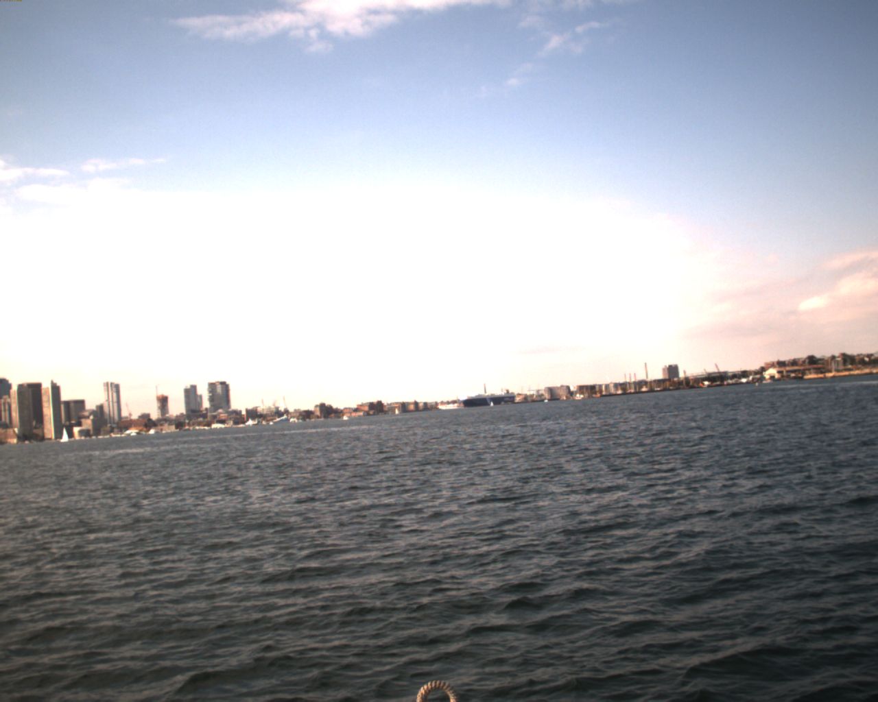
Look at Camera Data#
imd = await getBlob(client, context.userId, x9_de[0].id)
IMG_PATH='pyconvertimg.jpg'
with open(IMG_PATH, 'bw') as f:
    f.write(imd)

img = PILImage.open(IMG_PATH)
Image(filename=IMG_PATH)

Look at Radar Data#
rde = filter((lambda s: 'radar' in s.label), x9_de)
for rd in rde:
    print(rd)
<BlobEntry(label=radar_mkd_full,label=radar_mkd_full,id=6751eb5f-0475-4c24-a4e7-383109e59346)>
<BlobEntry(label=radar_img,label=radar_img,id=c8b00c48-4659-4437-b1e6-743b0c4be5bb)>
<BlobEntry(label=radar_pointcloud,label=radar_pointcloud,id=82a12130-1e4e-46d0-992a-7cac5708b7ab)>
As PointCloud#
rde = filter((lambda s: 'radar_pointcloud' in s.label), x9_de)
bE = next(rde)
print(bE)

radar_blob = await getBlob(client, context.userId, bE.id)
radar = json.loads(radar_blob)

print("Number of points: ",len(radar))
radar[0:10]
<BlobEntry(label=radar_pointcloud,label=radar_pointcloud,id=82a12130-1e4e-46d0-992a-7cac5708b7ab)>
Number of points:  643
[[-35.46592, 855.8134],
 [-119.02202, 484.61365],
 [216.1004, -631.304],
 [-158.5043, 830.0785],
 [-584.9095, -359.17392],
 [220.96115, 580.76575],
 [241.97108, 534.7688],
 [182.0528, -661.80194],
 [216.6408, 520.7562],
 [131.30196, -597.5646]]
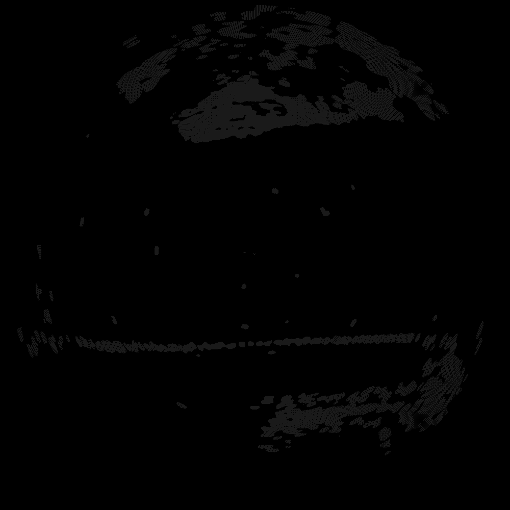
Radar To Image#
rde = filter((lambda s: 'radar_img' in s.label), x9_de)
bE = next(rde)
print(bE)

imd = await getBlob(client, context.userId, bE.id)
IMG_PATH='pyconvertimg.jpg'
with open(IMG_PATH, 'bw') as f:
    f.write(imd)

img = PILImage.open(IMG_PATH)
Image(filename=IMG_PATH)
<BlobEntry(label=radar_img,label=radar_img,id=c8b00c48-4659-4437-b1e6-743b0c4be5bb)>

Adding More Data#
Once you have a piece of data that is pertinant for storage, you can simply add it
Note these adds won’t work since userId=
examples@navability.iohas public read-only access, but requires authentication for write access.
# WRITING CHANGES WONT WORK WITHOUT AUTH for userId examples@navability.io
unique_id = await addBlob(client, "radar_pointcloud", cloudDens)
mime = "application/json/octet-stream"
addBlobEntry(
    client,
    context,
    "x9",
    unique_id,
    "radar_pointcloud",
    mime
)
The platform allows users to have various security/access levels as a particular application requires.
Building the Map with/without GPS#
A major emphasis of this tutorial is highlighting the importance of robust navigation from all sensors and data sources, while knowing that each sensor has it’s own problems and is unlikely to work perfectly 100% of the time – e.g. GPS fails under bridges when being jammed, cameras fail when the sun or reflections are in the field of view, and radar cross section detections and shadows can vary significatnly. By embracing non-Gaussian / multimodal data processing challenges head on, we are able to add significant value to the ease and robustness with which the necessary localization / mapping / tracking solutions that need to be developed.
Pull two radar sweeps and show a slice of the correlation maps from ScatterAlignPose2 – discuss.
Factors in the Session#
print(await listFactors(client, context))
['x0x4f_843d', 'x0f_ca58', 'x279x284f1', 'x274x279f1', 'x269x274f1', 'x264x269f1', 'x259x264f1', 'x254x259f1', 'x249x254f1', 'x244x249f1', 'x239x244f1', 'x234x239f1', 'x229x234f1', 'x224x229f1', 'x219x224f1', 'x214x219f1', 'x209x214f1', 'x204x209f1', 'x199x204f1', 'x194x199f1', 'x189x194f1', 'x184x189f1', 'x179x184f1', 'x174x179f1', 'x169x174f1', 'x164x169f1', 'x159x164f1', 'x154x159f1', 'x149x154f1', 'x144x149f1', 'x139x144f1', 'x134x139f1', 'x129x134f1', 'x124x129f1', 'x119x124f1', 'x114x119f1', 'x109x114f1', 'x104x109f1', 'x99x104f1', 'x94x99f1', 'x89x94f1', 'x84x89f1', 'x79x84f1', 'x74x79f1', 'x69x74f1', 'x64x69f1', 'x59x64f1', 'x54x59f1', 'x49x54f1', 'x44x49f1', 'x39x44f1', 'x34x39f1', 'x29x34f1', 'x24x29f1', 'x19x24f1', 'x14x19f1', 'x9x14f1', 'x4x9f1']
We can look a bit closer at one of the radar odometry factors:
f_x4x9 = await getFactor(client, context, "x4x9f1")
print(f_x4x9)
<Factor(label=x4x9f1,variables=['x4', 'x9'])>
The results from the line above shows a “data” value which in this particular case is a base64 encoded string. That field contains the data for a Caesar.ScatterAlignPose2 factor – also shows by:
f_x4x9.fnctype
'ScatterAlignPose2'
Aligning Radar PointCloud Maps#
To learn more, the factors as well as SLAM solver code is all open-source at JuliaRobotics/Caesar.jl. See the ScatterAlignPose2 factor code
Bring your own Visualizer (BYOV)#
We expect most applications already have a dedicated visualizer techonology choice, and this is good. The localization and mapping processing here is focussed on providing robust and distributed results which can be incorporated into existing visualization frameworks.
Basic awareness, App Geometric Visualization#
To make this tutorial accessible, we show the Marine Case study data with the NavAbility App, which provides a basic 2D visualizer to get a basic understanding of the data:
MapVizApp(context)
Next Steps#
If you have interest in NavAbility and what our technology can do, please reach out via Slack or info@navability.io.
Query spatial relationships,#
What is here there, or nearby
What might see this target
Find Boats in Camera Data#
Pull image data,
Process camera image with user side needs,
Track Boats in the Radar Data#
Combining Camera / Radar info Back into Factor Graph#
Dummy stub for uploading data back (not allowed under guest, please sign up for write access to a session)
Pull all this data into the factor graph and ask for a new solve


