Tutorial 4, Leveraging (Contradictory) Prior Data#
API Version: Python NavAbilitySDK.py
YouTube Walk Through Video:#
You can follow along with a YouTube walk through recording of this Tutorial notebook:
Applications Leveraging Data and Detecting Discrepancies#
Many industrial equipment/tools/robotics today are constrained to very rigid automation regimes. The following applications will be disrupted by navigation-affordance technology:
Reconfiguring manufacturing automation such as picking or packing using both asynchronous measurements and user desired programming,
Enhanced automation in surveyor Total Stations for lowering operational costs on construction sites,
Validation of “as-designed” vs. “as-built” in construction using design plans as affordances,
Metrology in manufacturing verification of part dimensions based on “as-designed” 3D solid models,
Rapid localization of underwater robotics in obscure environments using prior maps of semi-known environments,
e.g. relative navigation to known subsea infrastructure in energy or aquaculture,
Discrepancy detection through robotic inspection but detecting contradictions between intended and robotically mapped,
e.g. kelp farming installation status check that growth lines are not broken,
And many more.
This tutorial shows how prior data can be used to support as well as constrain robotic state-estimation tasks, while also gaining robustness to contradictory data. This tutorial will show how to combine prior and new measurement data through multi-hypothesis robustness.
Beyond “Brute-Force” Automation while Retaining Prior Knowledge#
To ground this tutorial, we take an example from production/manufacturing. Robotic factory lines are often difficult to reconfigure – i.e. are inflexible. Developing more reactionary robotic systems based on real-time sensor data is challenging. One of the critical needs for application specialists is an ability to expand robotic operations beyond rigid “brute force” (open-loop) automation whereby the human can incorporate/restrain a robot with better judgement (i.e. prior knowledge).
Conventional manufacturing and warehouse automation technologies operate via “brute force” or “playback” control strategies where robot operations follow a very narrow preprogrammed path. One of the major challenges in AI development for manufacturing and warehouse applications is to make the high value robotic equipment more flexible / reconfigurable so that the systems can more rapidly be reconfigured between different tasks.
One of the key challenges to expanding the automation software capabilities requires a balance between
programming the robot with human readible prior information about the task; as well as
letting the robotic automation handle more of the fine grain numerical operations relating to the task at hand.
The figure below shows a motivational example where prior knowledge—i.e. the corners of a rectangle and door opening—is to be used for robotic mapping operations.

The figure above illustrates some robotic equipment (a.k.a. the robot) which must be localized relative to a known rectangular shape. For simplicity, we introduce the door orientation as the only ambiguity which must be mapped by the robot – i.e. we know there is a door, but have not yet verified the hinging orientation.
The challenge of this tutorial is localizing and mapping the robot relative to the object as efficiently as possible, and have the solution be robust to possibly contradictory prior data. For the sake of illustration, we simplify the possible contradiction to the door orientation only, and invite the interested reader to see the NavAbility Construction Application example and associated publications for a more elaborate discussion on navigation-affordances.
Prior (Contradictory) Data#
This tutorial will demonstrate through a simplified example how prior (contradictory) data can be leveraged in a localization and mapping solution using factor graphs. We want to pre-load our robotic system with some basic information about the environment in which it will be operating so that it can more easily resolve it’s position and navigate around.
Room with a Door#
Prior info:
A rectangular room with the 4 corners as defining known navigation affordances,
An orientation sensitive door affordance which should* be hinged on the left side (which is buried in the data as an easter egg for the solver to discover as valid or contradictory).
ICRA Survey#
Thanks for doing our tutorials! We really want to make sure this is valuable for you.
This quick 2 minute survey will help us improve them for next year’s workshop.
Import Packages#
The first step load all the necessary packages, as listed in code blocks hereafter. The following commented code block is only necessary if your environment does not have the necessary packages installed for whatever reason (uncomment and run once if package are not installed).
# # ONLY IF REQUIRED, Install a pip package in the current Jupyter kernel
# import sys
# !{sys.executable} -m pip install navabilitysdk
from navability.entities import *
from navability.services import *
from uuid import uuid4
import asyncio
import numpy as np
We will also use the following door orientation printout function
def printHingedDoor(ornt, msg="resolved"):
  if np.abs(ornt) < np.pi/2:
    print('Door affordance %s as left hinged' % msg)
  else:
    print('Door affordance %s as right hinged' % msg)
Build a Multi-hypothesis Factor Graph#
We start with an empty factor graph object, which is created with default solver parameters.
# also create a client connection
client = NavAbilityHttpsClient()
# a unique userId:robotId
context = Client("guest@navability.io", "SDKpy_" + str(uuid4())[0:4], "Tutorial4_" + str(uuid4())[0:4])
Also a few basic noise parameters
prior_distr= np.power(np.diag([0.1, 0.1, 0.01]),2)
dual_distr= np.power(np.diag([0.5, 0.5, np.sqrt(np.pi)]),2)
Loading Known Prior Data#
Next, add to the factor graph the four corner prior knowledge about the room, namely c0, c1, c2, c3, each with their expected location in the world via PriorPose2 unary factor:
result_ids = []
result_id = await addVariable(client, context, "c0", VariableType.Pose2)
result_ids.append(result_id)
result_id = await addVariable(client, context, "c1", VariableType.Pose2)
result_ids.append(result_id)
result_id = await addVariable(client, context, "c2", VariableType.Pose2)
result_ids.append(result_id)
result_id = await addVariable(client, context, "c3", VariableType.Pose2)
result_ids.append(result_id)

result_id = await addFactor(client, context, ["c0"], PriorPose2(Z=FullNormal(mu=[0.,0, 0], cov=prior_distr)))
result_ids.append(result_id)
result_id = await addFactor(client, context, ["c1"], PriorPose2(Z=FullNormal(mu=[20.,0, np.pi/2], cov=prior_distr)))
result_ids.append(result_id)
result_id = await addFactor(client, context, ["c2"], PriorPose2(Z=FullNormal(mu=[20.,10, np.pi], cov=prior_distr)))
result_ids.append(result_id)
result_id = await addFactor(client, context, ["c3"], PriorPose2(Z=FullNormal(mu=[0.,10, -np.pi/2], cov=prior_distr)))
result_ids.append(result_id)
Also add the prior information regarding the door, and note for this simplified tutorial is using two affordance variables. Two variables is part of the affordance-duality construct where contradictions between prior known and ultimately discovered data can manifest in either the prior or dual variables, respectfully:
result_id = await addVariable(client, context, "door_prior", VariableType.Pose2)
result_ids.append(result_id)
result_id = await addVariable(client, context, "door_dual", VariableType.Pose2)
result_ids.append(result_id)

result_id = await addFactor(client, context, ["door_prior"], PriorPose2(Z=FullNormal(mu=[20., 4, 0], cov=prior_distr)))
result_ids.append(result_id)
result_id = await addFactor(client, context, ["door_dual"], PriorPose2(Z=FullNormal(mu=[20., 4, np.pi], cov=dual_distr)))
result_ids.append(result_id)
Solving the Room-only Graph#
Let’s make sure our prior data makes sense by solving the factor graph with the available data:
# wait for graph modifications to complete
await waitForCompletion(client, result_ids)

# request a solve
solve_request = await solveSession(client, context)
print('running solve...')
While the solve is running, let’s look so long at the factor graph so far, and look at the map thereafter…
The Room-only Graph Structure#
The basic room structure in the factor graph is also of interest. Let’s go ahead and look at what the graph structure looks like:
# Click on the generated factor graph graphic to open NavAbility App visualization
GraphVizApp(context, variableStartsWith="")
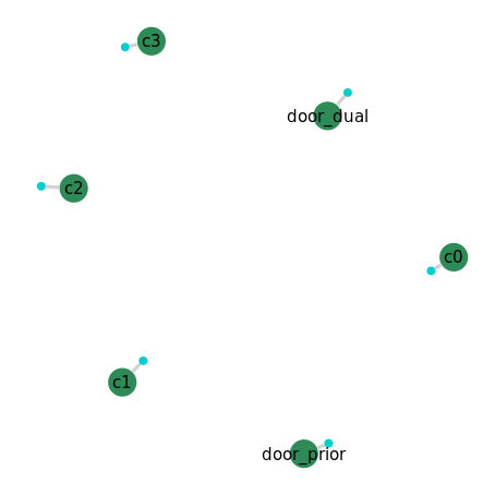
The graph plot above shows the simple factor graph so far, where four corner and dual door variables each have a prior factor. We are now ready to introduce new robotic measurements into the factor graph.
Map of Prior Data#
After completing the earlier solve, we can use the NavAbility WebApp to visualize the numerical values of the variables in the graph.
# Give it a few seconds JIT compiling during first run.
await waitForCompletion(client, [solve_request], maxSeconds=180)

# Click on the generated factor graph graphic to open NavAbility App visualization
MapVizApp(context)
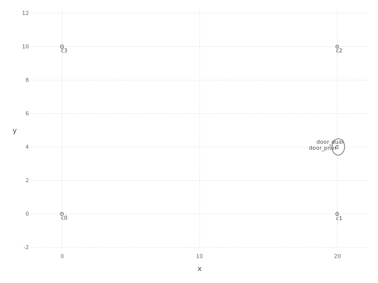
The plot shows the four corners as a rectangle between (0,0) and (20,10), as well as a door at (20,4). We also confirm the door prior data orientation which to the best of our current knowledge is left hinged:
door = await getVariable(client, context, "door_prior")
printHingedDoor(door.ppes["default"].suggested[2],"prior")
Door affordance prior as left hinged
Add Robotic Measurements (multihypo=)#
We would like to localize our robotic system relative to the available prior data above. The first thing the robot does is measure one of the corners relative to it’s own position (i.e. a relative, not global, measurement). Since we do not know which of the corners this measurement relates to, we will use the multihypo= keyword with equal 1/4 probability to each of the four known corners:
# add first pose variable
result_id = await addVariable(client, context, "x0", VariableType.Pose2)

# add multihypo factor to corner affordances
result_id = await addFactor(client, context,
                        ["x0", "c0", "c1", "c2", "c3"],
                        Pose2Pose2(Z=FullNormal(mu=[-2.,-2, 0], cov=np.power(np.diag([0.5, 0.5, 0.05]),2))),
                        multihypo=[1.0, 0.25, 0.25, 0.25, 0.25])

await waitForCompletion(client, [result_id])
Above we first added a new robot ‘pose’ variable x0. We then added a relative Pose2Pose2 factor which represents a rigid transform between the robot and the measured corner. Note, the measurement is local to the robot (i.e. not a global metrology-type measurement). Also note that the Pose2Pose2 factor is usually binary between two variables but now, with the multihypo= keyword, is associated with five variables. The first is the robot pose x0 with 100% certainty, while the next four corner affordance variables have fractional association certainty of 25% each.
Solve and Visualize the Multi-hypo Factor Graph#
Let’s start a new solve and look at the factor graph structure while the computation is running:
# request a new solve
solve_request = await solveSession(client, context)
print('running solve...')
They multi-hypo factor is represented in the factor graph as any other n-ary factor
# Click on the generated factor graph graphic to open NavAbility App visualization
GraphVizApp(context)
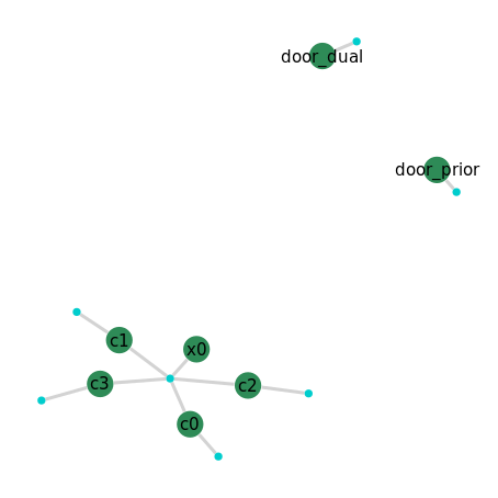
Let’s recap what the factor represents and what we are expecting to see. We know there are four corners to a room and we have one relative measurement to a corner. Therefore, the robot should be relatively positioned to one of the four known corners – i.e. we expect to see a multi-modal posterior belief estimate on the robot pose x0. Let’s plot the numerical results to see:
# wait for solve to complete...
await waitForCompletion(client, [solve_request], maxSeconds=180)

# Click on the generated factor graph graphic to open NavAbility App visualization
MapVizApp(context)
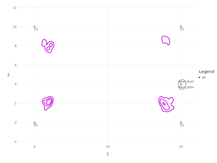
On the NavAbility App visualization, remember to enable the SHOW BELIEF button to see the underlying variable posterior belief estimates.
As predicted, there are four separate modes in the posterior marginal estimate of x0, one nearby each of the four known corners of the room. Note that each of these modes also have a marginal belief over the orientation of the robot which corresponds to the relative transform to the measured corner.
The critcal point here is that even though the factor graph does not have a unimodal solution, we are able to perform a solve on the graph and recover the correct non-Gaussian marginal posterior result.
Robot Moves to Position x1#
The next step towards mapping while localizating the robot relative to prior data is moving the robot and making more measurements. To get to the second position, we move the robot forward by 2 units and rotate clockwise (around positive z) by 90deg; this transform is captured in another rigid transform Pose2Pose2 factor to a new variable x1. Once at x1 the robot makes a second corner measurement for which we again don’t know the association:
result_id = await addVariable(client, context, "x1", VariableType.Pose2)

result_id = await addFactor(client, context,
                            ["x0", "x1"],
                            Pose2Pose2(Z=FullNormal(mu=[4.,0, np.pi/2], cov=np.power(np.diag([0.5, 0.5, 0.05]),2))),
                            nullhypo=0.5)

result_id = await addFactor(client, context,
                            ["x1", "c0", "c1", "c2", "c3"],
                            Pose2Pose2(Z=FullNormal(mu=[-2.,-4, 0], cov=np.power(np.diag([0.5, 0.5, 0.05]),2))),
                            multihypo=[1.0, 0.25, 0.25, 0.25, 0.25])

await waitForCompletion(client, [result_id])
Note, that even though we know this second corner measured is a different corner than what we measured first, we lazily added the new corner measurement again as a four way equal multihypo= uncertainty. We help the solver a little bit with this by allowed a bit more freedom in the solution (i.e. an additional source of entropy), but also stating that the interpose measurement might not be wholly correct – and we do this by including nullhypo=0.5.
We are therefore giving the factor graph solver less information than we actually have available. Let’s solve the graph again and see what it finds:
# request a new solve
solve_request = await solveSession(client, context)
print('running solve...')
# wait for solve to complete
await waitForCompletion(client, [solve_request], maxSeconds=180)

# Click on the generated factor graph graphic to open NavAbility App visualization
MapVizApp(context)
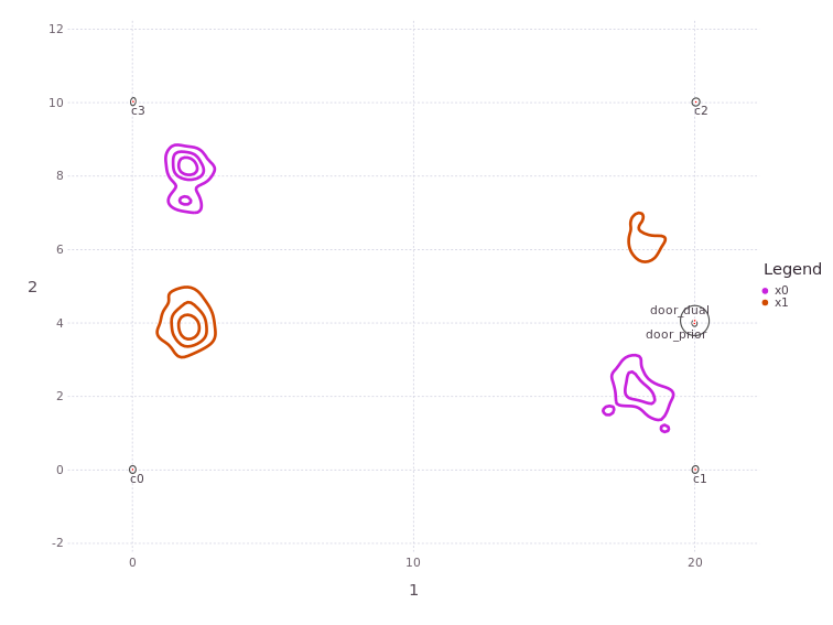
In the App visualization, remember to use the SHOW BELIEF button to see the underlying variable beliefs.
You should see the marginal posterior belief for pose x0 has reduced to two of the previous four modes, and the new x1 pose also having two associated modes from the relative factor. Therefore, the factor graph solution currently has two likely hypotheses contained within the numerical solution:
Mode 1 starts with
x0at(2,8)down tox1at(2,4)in affordance (rectangle coordinates), orMode 2 starts with
x0at(18,2)up tox1at(18,6).
Robot Moves to Position x2#
We move the robot forward by 16 units until a new boundary is detected, and add the new pose variable x2. A corner is again measured, and we again lazily add the Pose2Pose2 measurement to the new corner as a multihypo= factor at 1/4 association probability to any of the four prior known corners. Strictly speaking, the factor graph builder can already deduce that the new corner measurement is likely only one of two corners from the prior data, however, the point of this tutorial is to show that the factor graph builder’s job is being simplifiedy by a more capable back-end factor graph solver. So the new corner measurement factor is added in a lazy fashion:
result_id = await addVariable(client, context, "x2", VariableType.Pose2)

result_id = await addFactor(client, context,
                            ["x1", "x2"],
                            Pose2Pose2(Z=FullNormal(mu=[16.,0, 0], cov=np.power(np.diag([0.5, 0.5, 0.05]),2))))


result_id = await addFactor(client, context,
                            ["x2", "c0", "c1", "c2", "c3"],
                            Pose2Pose2(Z=FullNormal(mu=[2.,-4, np.pi/2], cov=np.power(np.diag([0.5, 0.5, 0.05]),2))),
                            multihypo=[1.0, 0.25, 0.25, 0.25, 0.25])

# wait for graph modifications to complete
await waitForCompletion(client, [result_id])
We start a new solve and take a look at the current graph structure:
# request a new solve
solve_request = await solveSession(client, context)
print('running solve...')
# Click on the generated factor graph graphic to open NavAbility App visualization
GraphVizApp(context)
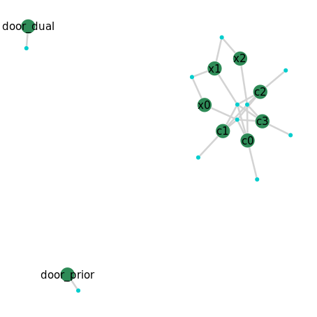
We see three corner measurements that could each be associated with any of the four prior corner affordances, (c0,c1,c2,c3). We also see the three new poses (x0,x1,x2) connected by two relative factors. The dual door affordance variables have not yet been sighted by the robot and only have prior factors at this time.
As the latest graph solve completes, we again and look at the numerical results:
# wait for solve to complete
await waitForCompletion(client, [solve_request], maxSeconds=180)

# Click on the generated factor graph graphic to open NavAbility App visualization
MapVizApp(context)
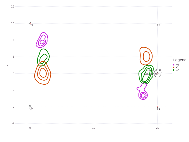
We find there are still two modes in each of the posterior marginal beliefs on the three poses (x0,x1,x2) which represent two hypotheses of how the robot is moving relative to the overall rectangular affordance.
The Robot Senses the Door!#
The last measurement made by the robot is to the door affordance, which is sensed to be 2 units ahead of the robot and to have a relative orientation to pose x2 of 180deg.
Final Graph Structure#
While the solve is porcessing, we can look at the final factor graph structure a last time, where we note that all variables are now interconnected by a series of prior and new measurement data. Building the factor graph was pretty easy, and the factor graph solver cranked through the numbers to untangle a multi-hypothesis mapping while localizing problem.
# Click on the generated factor graph graphic to open NavAbility App visualization
GraphVizApp(context, variableStartsWith="")
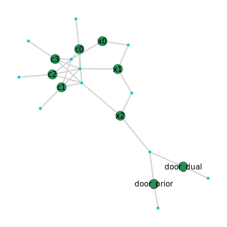
To simplify plotting, let’s look at just the three pose variables:
# wait for solve to complete
await waitForCompletion(client, [solve_request], maxSeconds=180)
# Click on the generated factor graph graphic to open NavAbility App visualization
MapVizApp(context, variableStartsWith="x")
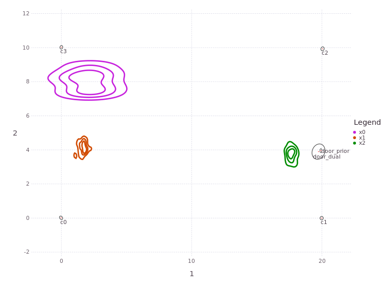
Re-solve to ensure Stable Unimodal Result#
Owing to the earlier nullhypo=0.5 on the factor between x0 and x1, it might be necessary to do a second solve to capture unimodal only beliefs. Simply run another solve and watch the numerical results converge.
# request a new solve
solve_request = await solveSession(client, context)
print('running solve...')
Only one hypothesis remains!#
Plotting again with both the affordance and pose information (resetting the variableStartsWith filter):
# Click on the generated factor graph graphic to open NavAbility App visualization
MapVizApp(context, variableStartsWith="")

Only one trajectory mode/hypothesis remains!
Resolved Correct Localization/Mapping Hypothesis#
The plot above shows a single hypothesis for pose locations (x0,x1,x2) of how the robot moved relative to the rectangular object. This resolution was extracted by making local measurements only and by leveraging prior data about the object. Resolving the robot position relative to the object did not require any global metrology measurements, and is furthermore able to resolve discrepancies between the prior anticipated navigation affordance models and the measured data. Let’s look at the door variables more closely…
Door Orientation is Contradictory#
The solver also resolved the correct :door_ orientation from local robot measurement data. We can see which door orientation was was found during measurement when comparing both the prior and dual variables. We use a small helper function to interpret the results:
door = await getVariable(client, context, "door_prior")
printHingedDoor(door.ppes["default"].suggested[2],"prior")
door = await getVariable(client, context, "door_dual")
printHingedDoor(door.ppes["default"].suggested[2])
Door affordance prior as left hinged
Door affordance resolved as right hinged
This indicates that the door affordance prior information is contradictory but the factor graph solution was correctly resolved during non-Gaussian inference to a stable, unimodal solution.
This concludes the tutorial on multi-hypothesis factors.
Conclusion and Next Steps#
Multi-hypothesis for Data Association#
This example shows one of four possible mechanisms by which non-Gaussian behavior can be introduced to a factor graph system. To simplify the tutorial, the measurements are assumed to be purely Gaussian and non-Guassian behavior is introduced through the multi-hypothesis data association mechanism. Other mechanisms shown in other examples can readily be added to this tutorial for a more intricate system.
The multi-hypothesis mechanism used in this tutorial also shows how the user can introduce discrete data association uncertainty into the estimation problem at the factor graph level. This approach is immediately applicable to loop-closures in SLAM, as was previously published – see Caesar.jl references here.
Contrast to Non-Gaussian Measurements#
Pay close attention to to the difference from Tutorial 2 where uncertainty about ambiguous data was marginalized into the measurements that was used to generate the factors. There is a major difference between non-Gaussian measurements in one factor vs. a unimodal factor with discrete uncertainty in association to variables – the crux of the matter is marginalization before or during inference.
The NavAbility platform and Caesar.jl solver allow the user to mix-and-match the four identified sources of non-Gaussian behavior in a single factor graph. This tutorial demonstrated one of those features using mapping of a navigation-affordance as the driving example.
On-Manifold Operations#
All the features describe above are computed on-manifold. For more information, see the Using Manifolds page in the Caesar.jl solver documentation.
Solving the Graph via the Bayes Tree#
The Caesar.jl solver uses the Bayes tree find the numerical solution for the factor graphs it’s solving. The open code has numerous features such as clique recycling a more. To learn more about the Bayes tree, see the Caesar.jl documentation page here.

